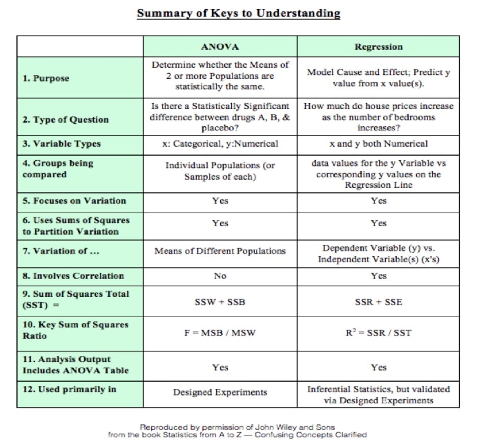
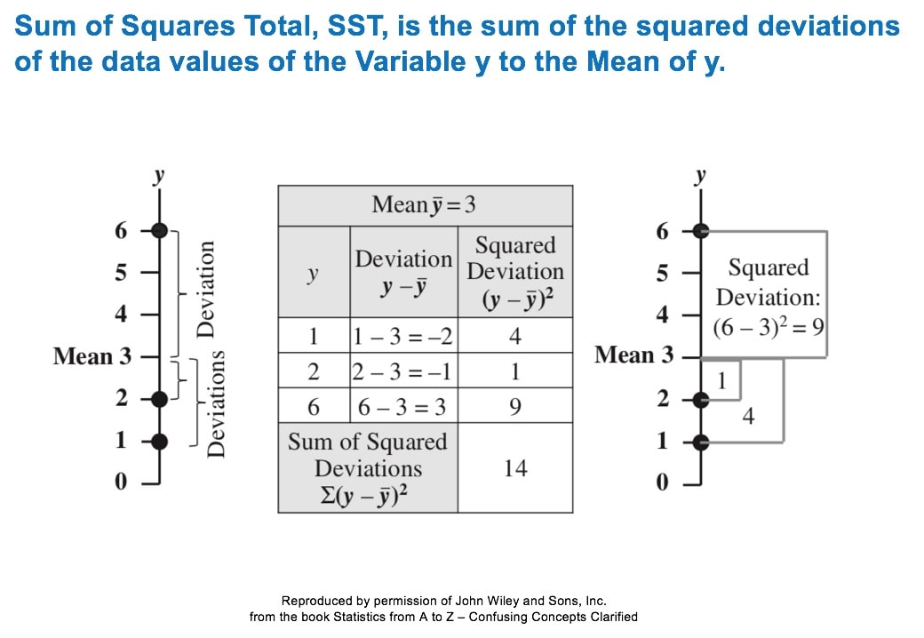
A method for performing 1-way (single factor) ANOVA can be illustrated in 7 steps, as shown in this concept flow diagram:

A Sum of Squares ​SS, is a measure of Variation within one Sample. In fact, it is the numerator in the formula for Variance. 

SSB and SSW  are described further in two of my recent Tips of the Week. And this 7-Step method is covered in my video: ANOVA -Part 3 (of 4): 1-Way aka Single Factor.

Step 1. Calculate the Sum of Squares (SS) for each Sample. 

SS is a measure of Variation within one Sample. In fact, it is the numerator in the formula for Variance. 
 
Step 2. Add all these up for all Samples to get the Sum of Squares Within.
​SSW 

SSW is a measure of the Variation within all the Samples. 

Step 3. Calculate the Overall Mean,  of all the data values in all Samples. 
Forget which data values go with which Samples, just put them all in one bucket and calculate the Mean. 
​
Step 4:  Sum up the squared differences between each Sample Mean (X-bar) and the Overall Mean  (X double bar),  to get Sum of Squares Between. 

Step 5: Calculate the Mean Sum of Squares Within (MSW) and Between (MSB). 
Sums of differences (like SSW and SSB) provide a gross measure of Variation. But it is often not meaningful to compare sums of different numbers of things. Averages (Means) are generally more meaningful than totals. So, we calculate MSW and MSB. 

Step 6: Perform an F-test 
The crux of ANOVA is comparing the Variation Within groups to the Variation Between (Among) groups. A group is a dataset like a population, process, or sample. The best way to do a comparison is to calculate a ratio. The F​​-statistic is a ratio of two Variances, MSB and MSW.

Note that this is a different concept from the usual F-test comparing Variances of two Samples. In that case, the Null Hypothesis would be that there is not a Statistically Significant difference between the Variances of two Samples. Although MSB and MSW have formulas like Variances, MSB and MSW contain information about the differences between the Means of the several groups. They contain no information about the Variances of the groups. 

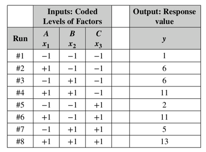
In the F-Test within ANOVA, the ANOVA Null Hypothesis is that there is not a Statistically Significant difference between MSB and MSW – that is, there is not a Statistically Significant difference among the Means of the several Groups. 

Step 7: 
Our choice of the Significance Level, Alpha, (most commonly 5%) determines the value of F-critical, and the F-statistic (calculated from the Sample data) determines the value of the Probability p. Comparing p to 𝛼 is identical to comparing F and F-critical.

If F ≥ F-critical (equivalently, p ≤ 𝜶), then there is a Statistically Significant difference between the Means of the groups. (Reject the ANOVA Null Hypothesis). 

If F < F-critical (p > 𝜶), then there is not Statistically Significant difference between the Means of the groups. (Accept/Fail to Reject the ANOVA Null Hypothesis). 

​In our Statistics Tip of the Week for April 6, 2017, we described the difference between Common Cause Variation in a process and Special Cause Variation. Common Cause Variation is like random noise in a process that is under control.  Special Cause Variation comes from external factors outside the process, like the effect that  the ambient temperature in a factory rising through most of the workday has on a chemical reaction. This type of factor is sometimes called a "Nuisance Factor" in the discipline of Design of Experiments. 
 
And, we said that any Special Cause Variation must be eliminated before one can attempt to narrow the range of Common Cause Variation. Narrowing the range of Common Cause Variation is a major objective of process improvement disciplines like Six Sigma. 
 
Factors -- the inputs -- are denoted by x's, and y is the output -- also known as the Response. Briefly, statistical software for Design of Experiments can provide us the number of trials ("Runs") to do and the levels of x for each trial. We might get test results that look like the following. (There is a lot to explain here, more than we can cover in this blog post).

Our Tip for April 12, 2018  said that Designed Experiments, together with Regression Analysis, can provide strong evidence of Causation. When we're doing these experiments, we are often not able to easily get rid of the Special Cause (Nuisance Factor) Variation, but we can try to reduce or eliminate its effect on the experiment.
 
A known Nuisance Factor can often be Blocked. To “Block” in this context means to group into a Block. By so doing, we try to remove the effect of Variation of the Nuisance Factor. In this example, we Block the effect of the daily rise in ambient temperature by performing all our experimental Runs within a narrow Block of time. And, if it takes several days to complete all the Runs, we do them all at a similar time of day in order to have the same ambient temperature. We thus minimize the the Variation in y caused by the Nuisance Factor. 

There can also be Factors affecting y which we don’t know about. Obviously, we can’t Block what we don’t know. But we can often avoid the influence of Unknown Factors (also known as “Lurking” Variables) by Randomizing the order in which the experimental combinations are tested. 
​
For example – unbeknownst to us – the worker performing the steps in a  process  may get tired over time, or, conversely, they might “get in a groove” and perform better over time. So, we need to Randomize the order in which we test the combinations of Factors.  Statistical software can provide us with the random sequences to use in the experiment. 

​Correlation does not imply Causation.

We can calculate a Correlation Coefficient, r, which will tell us that 2 Variables are strongly correlated. However, it doesn't tell us whether x causes y or vice versa. Or, there could be 3rd Variable which influences the behavior of both x and y.
 
Statistics alone can't tell us that. We need human subject matter experts to tell us what the real-world mechanisms and influencers are. 
 
If they confirm that there are likely mechanisms for the observed Correlation to be a cause and and an effect relationship, then we can use the data we have collected to develop a Regression Model to describe and size this cause and effect.
 
Are we done? No. We have to statistically demonstrate that the Regression Model describes what is actually happening. To prove the validity of the Regression Model, we cannot re-use the data we used to develop it.
 
We must go out and collect new data to test the validity of our Regression Model. We test our Regression Model with the new data, using methods described in the discipline of Design of Experiments. These experiments can give strong evidence of the  causation -- or not.

This is very much a simplification what goes on with several complicated and potentially confusing concepts. The book has 2 articles on Correlation, 5 articles on Regression, and 3 on Design of Experiments. Eventually, I hope to upload videos for each of these articles to my YouTube channel, "Statistics from A to Z -- Confusing Concepts Clarified". The videos page on this website will always show the latest status of the videos which are available and planned next to come. 

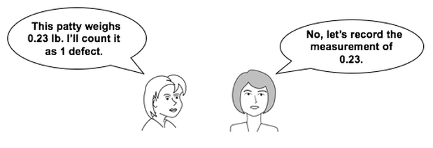
​In capturing data for statistical analysis, be sure to retain the information contained in measurement data, as opposed to reducing it to a count.
 
Let's say our company operates a process for producing meat patties for quarter-pound hamburgers. We want 0.25 pound burgers. Our specification limits call for all burgers to be between 0.24 and 0.26 pounds. Anything outside those limits is considered a defect.
 
We test the process quality by capturing a sample of data.  We could record the data by counting defects or by recording the actual measurement for each patty.

​When we measure 2 patties, weighing 0.23 and 0.21 pounds, if we only counted defects, we would record only the number 2 -- for 2 defects. You can see how this loses information contained in the measurements.
 
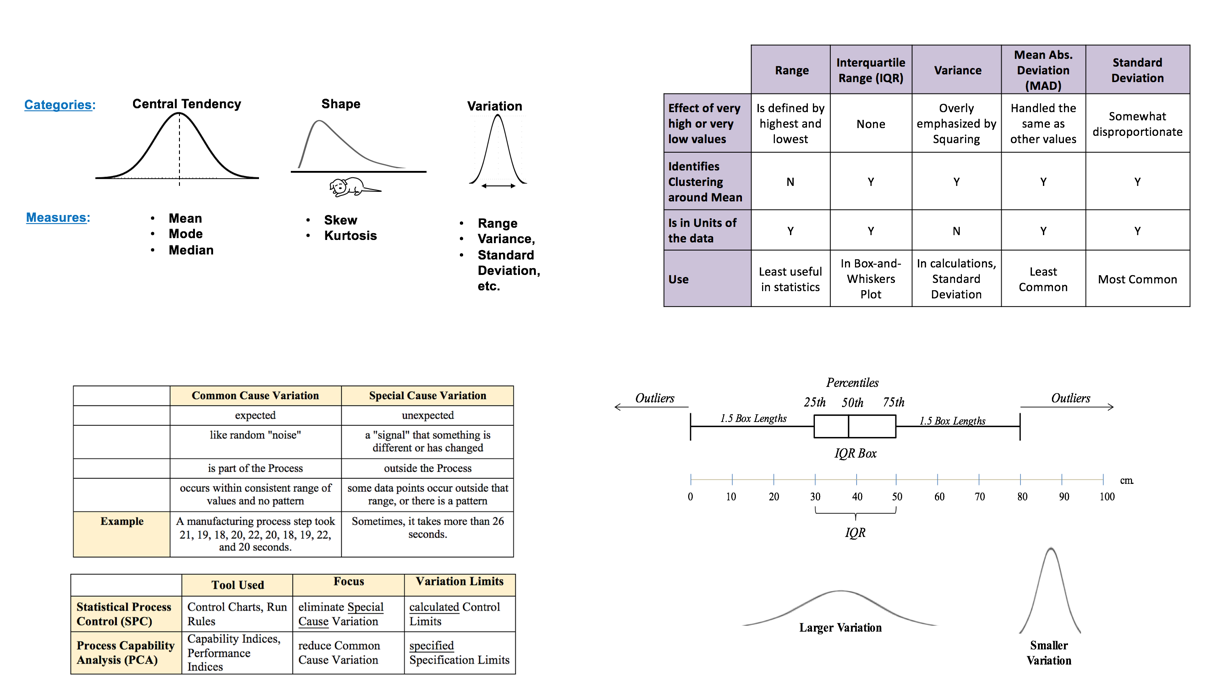
0.23 and 0.21 pounds are not equally defective. Counting them equally as 1 defect apiece makes for a less accurate assessment of process quality. 
 
So, to make the best use of the information contained in the data, we would do the analysis with measurement data, not counts. 

I just uploaded a new video. It is the first in a playlist on the concept variously known as "Variation", "Variability", "Dispersion", "Spread", and "Scatter". It gives an overview of the concept and compares and contrasts several measures of Variation: 

• Range
• Interquartile Range (IQR)
• Variance
• Mean Absolute Deviation (MAD), and
• Standard Deviation

Future additions to the playlist will cover in more detail:

• Sums of Squares
• Variance
• Standard Deviation
• Standard Error

These measures of Variation are for Populations and Samples. In addition, my book covers Variation in Processes, so in the future, there will be a separate playlist on these concepts:

• Statistical Process Control
• Control Charts Part 1
• Control Charts Part 2
• Process Capability Analysis