​In Regression, we attempt to fit a line or curve to the data. Let's say we're doing Simple Linear Regression in which we are trying to fit a straight line to a set of (x,y) data.

We test a number of subjects with dosages from 0 to 3 pills. And we find a straight line relationship,  y = 3x, between the number of pills (x) and a measure of health  of the subjects. So, we can say this.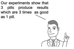

But we cannot make a statement like the following: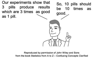

​This is called extrapolating  the conclusions of your Regression Model beyond the range of the data used to create it. There is no mathematical basis for doing that, and it can have negative consequences, as this little cartoon from my book illustrates.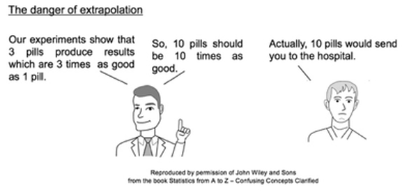

​In the graphs below, the dots are data points. In the graph on the left, it is clear that there is a linear correlation between the drug dosage (x) and the health outcome (y) for the range we tested, 0 to 3 pills. And we can interpolate between the measured points. For example, we might reasonably expect that 1.5 pills would yield a health outcome halfway between that of 1 pill and 2 pills.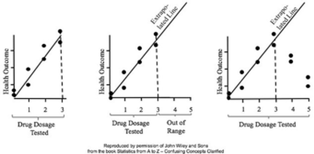

 For more on this and other aspects of Regression, you can see the YouTube videos in my playlist on Regression.  (See my channel: Statistics from A to Z - Confusing Concepts Clarified.

The Binomial Distribution is used with Count data. It displays the Probabilities of Count data from Binomial Experiments. In a Binomial Experiment,

• There are a fixed number of trials (e.g. coin flips)
• Each trial can have only 1 of 2 outcomes.
• The Probability of a given outcome is the same for each trial.
• Each trial is Independent of the others

There are many Binomial Distributions. Each one is defined by a pair of  values for two Parameters, n and p. n is the number of trials, and p is the Probability of each trial.

The graphs below show the effect of varying n, while keeping the Probability the same at 50%. The Distribution retains its shape as n varies. But obviously, the Mean gets larger.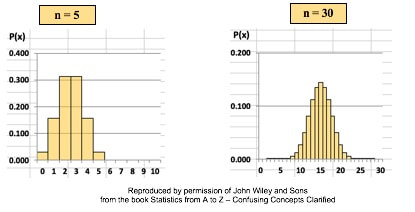 

​The effect of varying the Probability, p, is more dramatic.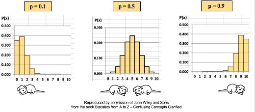

For small values of p, the bulk of the Distribution is heavier on the left. However, as described in my post of July 25, 2018, statistics describes this as being skewed to the right, that is, having a positive skew. (The skew is in the direction of the long tail.) For large values of p, the skew is to the left, because the bulk of the Distribution is on the right. 

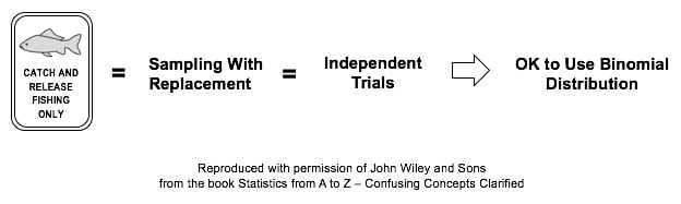One of the requirements for using the Binomial Distribution is that each trial must be independent. One consequence of this is that the Sampling must be With Replacement.

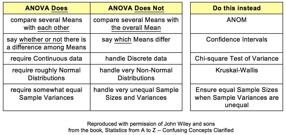
To illustrate this, let's say we are doing a study in a small lake to determine the Proportion of lake trout. Each trial consists of catching and identifying 1 fish. If it's a lake trout, we count 1. The population of the fish is finite. We don't know this, but let's say it's 100 total fish 70 lake trout and 30 other fish. 

Each time we catch a fish, we throw it back before catching another fish. This is called Sampling With Replacement. Then, the Proportion of lake trout is remains at 70%. And the Probability for any one trial is 70% for lake trout. 

If, on the other hand, we keep each fish we catch, then we are Sampling Without Replacement. Let's say that the first 5 fish which we catch (and keep) are lake trout. Then, there are now 95 fish in the lake, of which 65 are lake trout. The percentage of lake trout is now 65/95 =68.4%. This is a change from the original 70%.

So, we don't have the same Probability each time of catching a lake trout. Sampling Without Replacement has caused the trials to not be independent. So, we can't use the Binomial Distribution. We must use the Hypergeometric Distribution instead.

For more on the Binomial Distribution, see my YouTube video.

For more details on ANOVA, I have a 6-video playlist on YouTube.

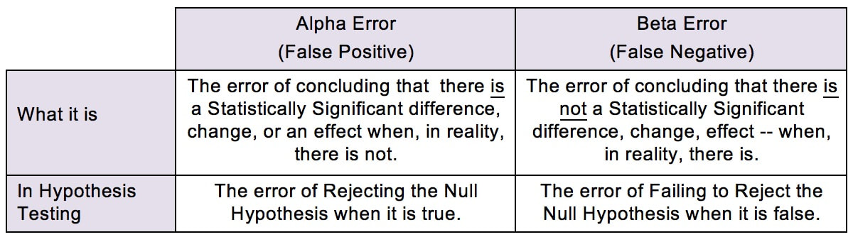
There are a number of see-saws (aka "teeter-totters" or "totterboards") like this in statistics. Here, we see that, as the Probability of an Alpha Error goes down, the Probability of a Beta Error goes up. Likewise, as the Probability of an Alpha Error goes up, the Probability of a Beta Error goes down.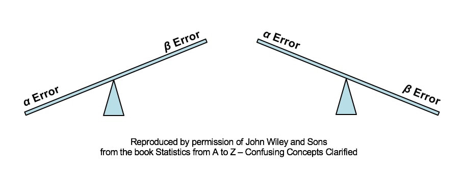

​This being statistics, it would not be confusing enough if there were just one name for a concept.  So, you may know Alpha and Beta Errors by different names:

• Alpha Error: false positive, type I error, error of the first kind
• Beta Error: false negative, type II error, error of the second kind

The following compare-and-contrast table should help explain the difference:

The see-saw effect is important when we are selecting a value for Alpha (α) as part of a Hypothesis test. Most commonly, α = 0.05 is selected. This gives us a 1 – 0.05 = 0.95  (95%) Probability of avoiding an Alpha Error.

Since the person performing the test is the one who gets to select the value for Alpha, why don't we always select α = 0.000001 or something like that?
​
The answer is, selecting a low value for Alpha comes at price. Reducing the risk of an Alpha Error increases the risk of a Beta Error, and vice versa.

There is an article in the book devoted to further comparing and contrasting these two types of errors. Some time in the future, I hope to get around to adding a video on the subject. (Currently working on a playlist of videos about Regression.) See the  videos page of this website for the latest status of videos completed and planned.

​Most users of statistics are familiar with the F-test for Variances. But there is also a Chi-Square Test for the Variance. What's the difference?

​The F-test compares the Variances from 2 different Populations or Processes. It basically divides one Variance by the other and uses the appropriate F Distribution to determine whether there is a Statistically Significant difference.

If you're familiar with t-tests, the F-test is analogous to the 2-Sample t-test. The F-test is a Parametric test. It requires that the data from both the 2 Samples each be roughly Normal.

The following  compare-and-contrast table may help clarify these concepts: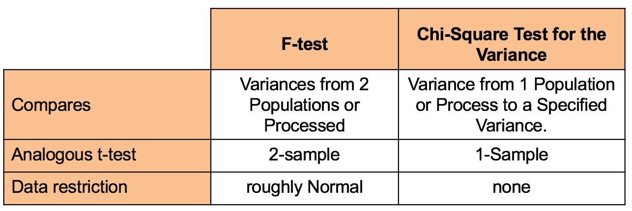

​Chi-Square (like z, t, and F) is a Test Statistic. That is, it has an associated family of Probability Distributions.
 
The Chi-Square Test for the Variance compares the Variance from a Single Population or Process to a Variance that we specify. That specified Variance could be a target value, a historical value, or anything else.
 
Since there is only 1 Sample of data from the single Population or Process, the Chi-Square test is analogous to the 1-Sample t-test.
 
In contrast to the the F-test, the Chi-Square test is Nonparametric. It has no restrictions on the data. 

Videos: I have published the following relevant videos on my YouTube channel, "Statistics from A to Z"

• F Distribution:  https://youtu.be/w1TvaQgoNCY 
• Chi-Square -- the Test Statistic and Its Distributions: https://youtu.be/RJMNkzuxOA4   
• t: the Test Statistic and Its Distributions: youtu.be/3GCJU_RCgoM    

There are 3 categories of numerical properties which describe a Probability Distribution (e.g. the Normal or Binomial Distributions).

• Center: e.g. Mean
• Variation: e.g. Standard Deviation
• Shape: e.g. Skewness 

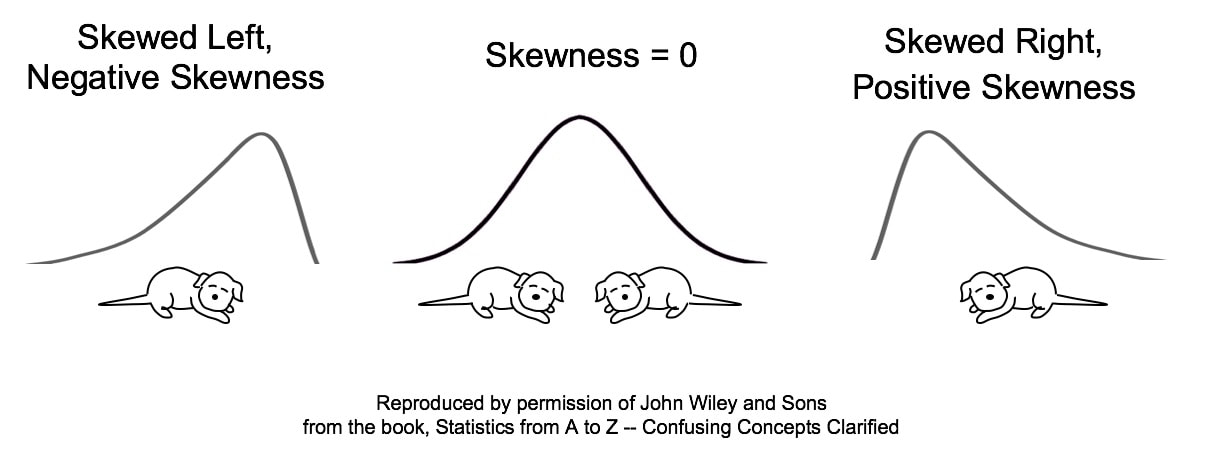Skewness is a case in which common usage of a term is the opposite of statistical usage. If the average person saw the Distribution on the left, they would say that it's skewed to the right, because that is where the bulk of the curve is. However, in statistics, it's the opposite. The Skew is in the direction of the long tail.
​
If you can remember these drawings, think of "the tail wagging the dog."

​Many folks are confused about this, especially since the names for these tests themselves can be misleading. What we're calling the "2-Sample t-test" is sometimes called the "Independent Samples t-test". And what we're calling the "Paired t-test" is then called the "Dependent Samples t-test", implying that it involves more than one Sample. But that is not the case. It is more accurate -- and less confusing -- to call it the  Paired t-test.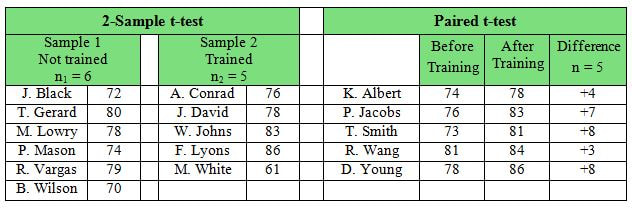

First of all, notice that the 2-Sample test, on the left, does have 2 Samples. We see that there are two different groups of test subjects involved (note the names are different) -- the Trained and the Not Trained. The 2-Sample t-test will compare the Mean score of the people who were not trained with the Mean score of different people who were trained.

The story with the Paired Samples t-test is very different. We only have one set of test subjects, but 2 different conditions under which their scores were collected. For each person (test subject), a pair of scores -- Before and After -- was collected. (Before-and-After comparisons appear to be the most common use for the Paired test.) 

Then, for each individual, the difference between the two scores is calculated. The values of the differences are the Sample (in this case: 4, 7, 8, 3, 8 ). And the Mean of those differences is compared by the test to a Mean of zero.

For more on the subject, you can view my video, t, the Test Statistic and its Distributions.      
​

Alpha, p, Critical Value, and Test Statistic are 4 concepts which work together in many statistical tests. In this tip, we'll touch on part of the story. The pictures below show two graphs which are close-ups of the right tail of a Normal Distribution. The graphs show the result of calculations in 2 different tests.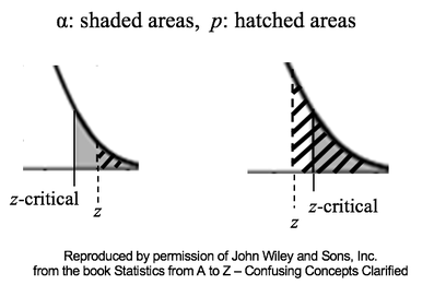

The horizontal axis shows values of the Test Statistic, z. So, z is a point value on this horizontal z-axis. z = 0 is to the left of these close-ups of the right tail. The value of z is calculated from the Sample data. 

• Note that the calculated z defines the boundary of a hatched area. The  hatched areas under the curve represent the value of the Cumulative Probability, p.
• And z-critical (the Critical Value of z) defines the boundary of the shaded area representing α.

 
For more on how these four concepts work together, there is an article in the book, "Alpha, p, Critical Value and Test Statistic -- How They Work Together". I think this is the best article in the book. You can also see that article's content on my YouTube video. There are also individual articles and videos on each of the 4 concepts. My YouTube Channel is "Statistics from A to Z -- Confusing Concepts Clarified".  

In ANOVA, Sum of Squares Total (SST) equals Sum of Squares Within (SSW) plus Sum of Squares Between. (SSB). That is, SST = SSW + SSB.  In this Tip, we'll talk about Sum of Squares Within, SSW. In ANOVA, Sum of Squares Within (SSW) is the sum of Variations within each of several datasets or Groups.

The following illustrations are not numerically precise. But, conceptually, they portray the concept of Sum of Squares Within as the width of the “meaty” part of a Distribution curve – the part without the skinny tails on either side. 

​Here, SSW = SS1 + SS2 +SS3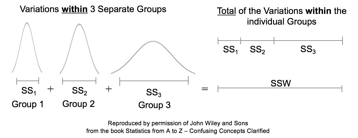

For more on Sums of Squares, see my video of that name: https://bit.ly/2JWMpoo .
For more on Sums of Squares within ANOVA, see my video, "ANOVA Part 2 (of 4): How It Does It: http://bit.ly/2nI7ScR .