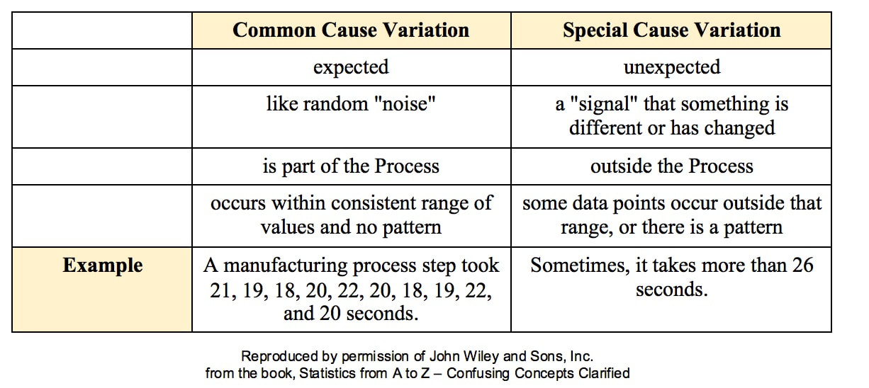
​My blog post of April 6, 2017 discussed how Control Charts and Run Rules are used to distinguish Common Cause from Special Cause Variation. Common Cause Variation is the usual, expected, random "noise" variation that all processes have. It occurs within limits and it exhibits no pattern. If all we have is Common Cause Variation, then we can begin implementing process improvement techniques to reduce this variation.

​But if the variation exceeds the limits in a Control Chart or if it exhibits patterns described in Run Rules, then the process in not in control. Special Cause Variation is in effect, and that needs to be addressed first.
 
There are a number of different types of Control Charts. For Discrete/ Count data (integers) here are the Control Charts to use. 

What's the difference between units and occurrences? Let's say we are inspecting shirts that we are manufacturing.  One shirt with 3 defects would count as 1 defective unit or 3 occurrences of defects.

For Continuous/ Measurement data (real numbers), use the following charts:

​p is the Probability of an Alpha (false positive) Error. The p-value is calculated as the area under the curve bounded by the Test Statistic value.  

As shown in the concept flow diagram above, the first thing we do is take the Sample data and calculate a value for the Test Statistic.  In this example, the value of the Test Statistic, z, is calculated to be 1.2.

​​Next, (illustrated here for a 1-tailed test), we plot the Test Statistic value on the horizontal axis of the Probability Distribution of the Test Statistic.  (For a 2-tailed test, we would plot 1/2 the value of z at the left and right ends sides of the curve. In this example, we would plot z/2 = 0.6 and -z/2 = -0.6).

The Test Statistic Value forms the boundary of an area under the curve extending outward from the Test Statistic value. Here we show a hatched area from z = 1.2 outward to infinity.
 
The hatched area under the curve is calculated as the Cumulative Probability of all points under the curve from z = 1.2 outward. This gives us the value for p.

For more on the concepts involved here, please see my videos:

• Test Statistic  https://youtu.be/2fz0STTfIIU
• p, the p-value https://youtu.be/vyX4m89VkyI
• Alpha, p, Critical Value and Test Statistic: How they work together. https://youtu.be/SAYGehjRZ8E

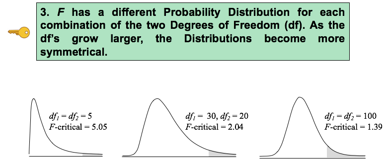
A new entry to the "Distributions" playlist on my YouTube Channel: ​​F Distribution. 

There are 4 Keys to Understanding this concept. Here's the third:

See the videos page on this blog for a status of videos completed and planned. 

In 2-Factor (aka "2-Way") ANOVA, we study the effect of 2 Nominal (named) Variables A and B, on the Dependent Numerical Variable y. (For more on Nominal (also known as "Categorical" Variables) see my blog post from November 23, 2016 .)

y = f(A,B) or y = f(A,B, AB)

A and B are the Factors influencing the value of y. "AB" -- which may or may not exist -- is the Interaction between A and B. It can be a 3rd Factor if it is Statistically Significant. 

In the example below,

• we start with y = f(A,B). y is a numerical measure of cleanliness.
• Factor A is the type of detergent. There are two values of A tested: "Detergent 1" and "Detergent 2".  Note that these values are names, since Factor A is a Nominal Variable.
• Factor B is the water temperature. There are three values of B tested: "Cold", "Warm" and "Hot". As you can see, Factor B is also a Nominal Variable.

We must use the WITH REPLICATION method of 2-Way ANOVA if there is a Statistically Significant Interaction.
 
But how do we know if there is? As my blog post of June 8, 2017  says, you can use a line chart to identify Interactions.  If the lines cross, that indicates an Interaction, and the With Replication method must be used. That method can determine if the Interaction is Statistically Significant.
 
In the left diagram below, neither type of detergent is affected by water temperature, so there is no Interaction between Factor A, detergent type, and Factor B, water temperature.  In the middle diagram, both detergents of Factor A are affected the same. Cleanliness is improved similarly with hotter water, no matter what detergent is used. So, again there is no Interaction. 

In the right diagram, they behave differently. Hotter water makes Detergent #1 more effective, but makes Detergent #2 less effective. The lines definitely cross, indicating a Statistically Significant Interaction. We'll need to perform a 2-Way ANOVA With Replication to make sure.
 
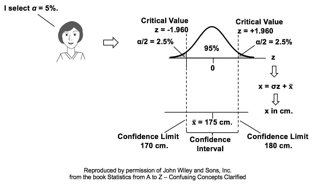
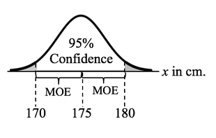
With the With Replication method, we replicate (repeat) the taking of measurements several times with different levels of each Factor (detergent type and water temperature). We need to use the discipline of Design of Experiments (DOE) to specify the number of Replications required and what values of each Factor comprise each Replication. The book has a 3-part series of articles on DOE, and I plan to eventually record videos on the subject.
 
For more on 2-Way ANOVA, both WIth and Without Replication, see my video:
ANOVA Part 4 (of 4) -- 2-Way (aka 2-Factor).        

In the July 18, 2017 Statistics Tip of the Week, we showed how a Confidence Interval is calculated. As illustrated in the concept flow diagram below,

• the tester selects a value for Alpha, the Significance Level.
• This, plus a Test Statistics Distribution, gives us 2 Critical Values for a 2-sided test.
• We convert these values into units of the data, x, giving us 2 Confidence Limits which define a Confidence Interval.

​Based on this, we might summarize the results of the test by saying "With a 95% Level of Confidence, we estimate the Mean height to be 175 centimeters, with a Margin of Error of plus or minus 5 cm."