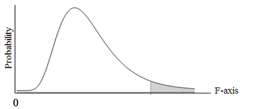
In the book's article on F, the first Key to Understanding is:

​A Test Statistic is one whose Distribution has known Probabilities. So, for any value of F (on the horizontal axis below), there is a known Probability of that value occurring. That Probability is the height of the curve above that point. 

More importantly, we can calculate the area under the curve beyond any value of F. This gives us a Cumulative Probability (such as p, the p-value) which we can use to compare to the Significance Level, 𝛼 (also a Cumulative Probability), in various types of analyses in Inferential Statistics. A Cumulative Probability is usually depicted as a shaded area under the curve.

F is Continuous Distribution. Its curve has a smooth shape, unlike the histogram-like shape of Discrete Data Distributions. However, it can work with Samples of Discrete data. The ratio of the Variances of two sets of Discrete Data is Continuous.
​
F is the ratio of Two Variances. To keep things simple, the larger Variance is entered as the numerator, and the smaller is the denominator, except for ANOVA, where the numerator and denominator are specified.

​where s1 and s2 are the symbols for the Standard Deviations of a Samples 1 and 2, respectively. The square of any Standard Deviation is a Variance. 

​In ANOVA: F = MSB/MSW,

where MSB is the Mean Sum of Squares Between and MSW is the Mean Sum of Squares Within. Both are special types of Variances. My previous blog post talks about SSW, which is used to calculate MSW.

For more on F, see my video: F Distribution. There is also a video on Test Statistics. There is also a playlist with several videos on ANOVA and related concepts . You can always get the latest status of my videos on the "Videos" page of this website.

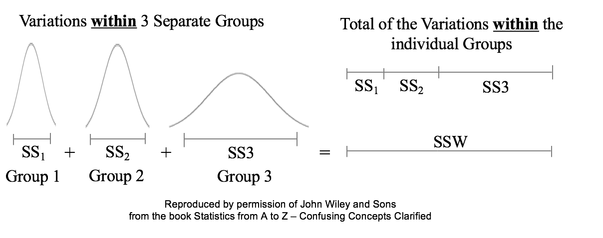
Sums of Squares are measures of variation; there are a number of different types. Our Tip of the Week for Dec. 21, 2017 described Sum of Squares Total (SST), which is used in Regression.  Sum of Squares Within (SSW) is used in ANOVA.  Sum of Squares Between (SSB) is also used in ANOVA, and it will be the topic of another Statistics Tip of the Week.
 
Sum of Squares Within, SSW, is the sum of the Variations (as expressed by the Sums of Squares, SS's) within each of several Groups (usually Samples).

​This is not numerically precise, but conceptually, one might picture SS as the width of the "meaty" part of a Distribution curve – the part without the skinny tails on either side.

​Sums of Squares Within, SSW, summarizes how much Variation there is within each of the Groups– by giving the sum of all such Variations.

​A comparatively small SSW indicates that the data within the individual Groups are tightly clustered about their respective Means. If the data in each Group represents the effects of a particular treatment, for example, this is indicative of consistent results (good or bad) within each individual treatment. "Small" is a relative term, so the word "comparatively" is key here. We'll need to compare SSW with SSB before being able to make a final determination.                                                                            
 
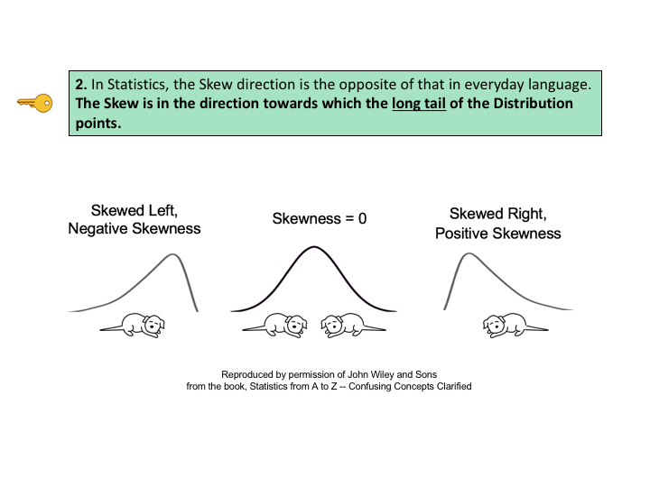
A comparatively large SSW shows that the data within the individual Groups are widely dispersed. This would indicate inconsistent results within each individual treatment. 

For more on the subject and related concepts see my video, ANOVA Part 2 (of 4): How it Does It.

New Video, Skew, Skewness,  uploaded to the book's channel.
For a list of available and planned videos, see the Videos page on this website.

"Statistics is the part of mathematics that even mathematicians don't particularly like." Alan Smith, Data Visual Editor, the Financial Times in London.
http://bit.ly/2DmPueD
 

​Randomness is likely to be representative, and Simple Random Sampling (SRS) can often be the most effective way to achieve it. But in certain situations, other methods such as Systematic, Stratified, and Clustered Sampling may have an advantage.
 
In our Tip of the Week for November 27, 2017, Stratified Sampling was described. This Tip is about Clustered Sampling. To perform Clustered Sampling,

1. Divide the Population or Process into small clusters (e.g. city blocks)
2. Select a Simple Random Sample of these clusters
3. Collect data from each unit within each cluster

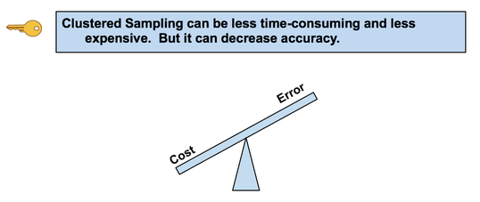
​Advantage: It can be less time-consuming and less expensive. For example, the Population is the inhabitants of a city, and a cluster is a city block. We randomly select an SRS of city blocks. 

​There is less time and travel involved in traveling to a limited number of city blocks and then walking door to door, compared with traveling to more-widely-separated individuals all over the city. Also, one does not need a Sampling Frame listing all individuals, just all clusters.
 
Disadvantage: The increased Variability due to between-cluster differences may reduce accuracy. 

Chi-Square is a Test Statistic; as such, it has a family of Distributions. There is a different Chi-Square Distribution for each value of Degrees of Freedom, df.

Commonly, Degrees of Freedom is the Sample Size minus 1. But this isn't always the case with Chi-Square. That will be covered in a future Tip of the Week. 

Here are some examples of how the Chi-Square Distribution varies as df increases. You might observe that the shape of the Chi-Square Distribution is similar to that of the F-Distribution. For more on the Chi-Square, its Distributions and Tests, see the book or this video.  

I just uploaded a new video.: https://youtu.be/3GCJU_RCgoM It's an addition to the playlist on Probability Distributions.

​Check out the "​Videos" page of this website for a list of completed videos and plans for upcoming videos.