Statistics Tip of the Week: F is a Test Statistic which is the ratio of two Variances.

In the book's article on F, the first Key to Understanding is:

​A Test Statistic is one whose Distribution has known Probabilities. So, for any value of F (on the horizontal axis below), there is a known Probability of that value occurring. That Probability is the height of the curve above that point.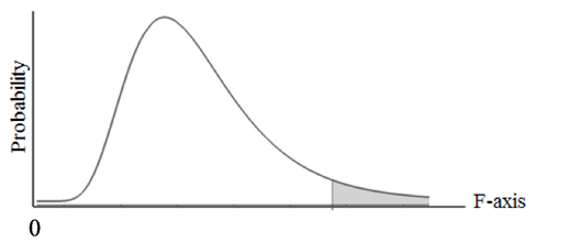 

More importantly, we can calculate the area under the curve beyond any value of F. This gives us a Cumulative Probability (such as p, the p-value) which we can use to compare to the Significance Level, 𝛼 (also a Cumulative Probability), in various types of analyses in Inferential Statistics. A Cumulative Probability is usually depicted as a shaded area under the curve.

F is Continuous Distribution. Its curve has a smooth shape, unlike the histogram-like shape of Discrete Data Distributions. However, it can work with Samples of Discrete data. The ratio of the Variances of two sets of Discrete Data is Continuous.
​
F is the ratio of Two Variances. To keep things simple, the larger Variance is entered as the numerator, and the smaller is the denominator, except for ANOVA, where the numerator and denominator are specified.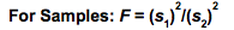

​where s1 and s2 are the symbols for the Standard Deviations of a Samples 1 and 2, respectively. The square of any Standard Deviation is a Variance. 

​In ANOVA: F = MSB/MSW,

where MSB is the Mean Sum of Squares Between and MSW is the Mean Sum of Squares Within. Both are special types of Variances. My previous blog post talks about SSW, which is used to calculate MSW.

For more on F, see my video: F Distribution. There is also a video on Test Statistics. There is also a playlist with several videos on ANOVA and related concepts . You can always get the latest status of my videos on the "Videos" page of this website.